Inhibition, Accuracy and Firing
Reused MNIST networks compare accuracy and excitatory firing rates with and without an inhibitory loop. Full-MNIST reference classifiers accompany a separate reduced-training-pool activity-ceiling sweep.
Abstract
We compared MNIST accuracy and excitatory firing in trained COBA and PING classifiers across activity ceilings, with three independent training seeds per frontier condition. Without a rate penalty in the reduced-pool study, PING reached 89.8% test accuracy at 16.6 Hz, versus 90.9% at 88.2 Hz for COBA. Additional single-seed probes measured cycle participation and input-coupling sensitivity. These comparisons neither establish a structural firing-rate floor nor isolate a benefit of gamma timing or measure energy use.
Results
Accuracy-rate activity ceilings
Full-MNIST reference classifiers reached mean final validation accuracies of 91.4% for PING and 95.3% for COBA (Figure 1A–C). In the separate reduced-training-pool comparison, at the unpenalised operating points, PING reached 89.8% at 16.6 Hz and COBA reached 90.9% at 88.2 Hz. These measurements do not establish a structural lower firing-rate limit (Figure 1D).

(A–B) Illustrative 200 ms COBA and PING rasters from final full-MNIST checkpoints for the same digit-0 example, seed 42; E spikes are black and I spikes red. (C) Full-MNIST validation accuracy over training, averaged across three seeds without uncertainty intervals. A–C use 54,000 optimization and 6,000 validation images. (D) Separate classifiers trained on 6,300 optimization and 700 validation images: test accuracy versus mean E firing rate across activity ceilings; means ± SEM over three seeds, unpenalised points starred. Numeric labels give ceiling values in hertz; the PING 25 Hz ceiling marker nearly coincides with its unpenalised star. These rates are test-set averages, not raster estimates. PING black and COBA red in panels C–D.
PING participation and frequency
PING participation varied from 0.16 to 0.26 and oscillation frequency from approximately 60 to 18 Hz. The approximation differed from measured E rate by up to 27.5%, so participation was not constant. PING accuracy spanned 81–90%; COBA fell from 89% to 62% as the ceiling tightened (Figure 2).

(A) PING participation, (B) PING gamma frequency, (C) E rate with the approximation and (D) accuracy across activity ceilings. Five penalised conditions per model, seed 42, 1000 test images each. The dashed curve in C is the approximation. These are individual-seed measurements, not across-seed estimates.
Input-coupling learning curves
Final validation accuracies were 76.5% / 76.6% / 76.8% / 76.6%, while final I rates were 5.6 / 5.8 / 5.6 / 5.6 Hz. The similar endpoints across these initializations do not prove basin attractivity (Figure 3).

PING learning curves for initial input-coupling means 0.05, 0.1, 0.3 and 0.9. Panels A–D show validation accuracy in that order; E–H show validation E (black) and I (red) rates in the same order. The rate ceiling is 1 Hz throughout; lines and shading show means ± SEM across seeds 42–44.
Inference input-scaling response
COBA’s penalty reached approximately 2 at . The empirical inhibitory-rate crossing marks a sampled transition, not a fitted bifurcation (Figure 4).

Seed-42 networks trained with a 1 Hz ceiling; input weights scaled at inference over 24 values, all other weights fixed. (A) Cross-entropy, (B) rate penalty, (C) their sum, (D) test accuracy with a dotted chance line, (E) E rate and (F) I rate; 1000 images per condition. PING black, COBA red. Dashed marks training; the dotted marker labelled denotes the empirical input scale 0.475 where I rate crosses 0.05 Hz, not a fitted bifurcation. Penalty and total-objective axes stop at 4.
Accuracy-rate input scaling
PING’s highest sampled accuracy was approximately 83%. At input scale , COBA reached approximately 63% at 8 Hz. This single direction of weight scaling does not map the full loss landscape (Figure 5).

Figure 4 replotted against mean E rate: (A) cross-entropy, (B) rate penalty, (C) their sum, (D) test accuracy, (E) I rate and (F) input-weight scale. Stars mark the trained points: PING 4.7 Hz and COBA 2.1 Hz.
Methods
We reused networks and learning histories from the exp022 — MNIST and reanalysed recorded inference measurements; no new training or simulation was performed.
Compute
-
Prepare digit inputs. Full-MNIST reference classifiers in Figure 1 A–C used all 60,000 official-training images, split into 54,000 optimization and 6,000 validation images. The activity-ceiling and input-coupling studies used a separate 7,000-image pool, split into 6,300 optimization and 700 validation images. Sampling and class-stratified splitting used seed 42. Pixels drove 784 Poisson channels at a 25 Hz maximum, for 200 ms with 0.1 ms steps.
-
Compare network configurations. Both conductance-based networks had 1,024 excitatory (E), 256 inhibitory (I), and 10 output leaky-integrate-and-fire neurons. Pyramidal-interneuron gamma (PING) enabled fixed E↔I coupling; COBA disabled it; E→E and I→I coupling were zero throughout. Only input and readout weights trained; class scores were mean pre-reset output membrane voltages. Voltage-gradient damping was 1,000 for both COBA and PING.
-
Train with activity ceilings. Networks trained for 50 epochs with AdamW (zero weight decay), learning rate , batch size 256, and gradient-norm clipping at 1. Cross-entropy was supplemented by:
Here counts excitatory neuron ‘s spikes in presentation , is the excitatory population, its size, its duration in seconds, and minibatch size. Rates and ceilings are in hertz; weights the dimensionless penalty . Six ceiling conditions (Training settings) and three seeds yielded 36 reduced-pool networks. Six separate full-MNIST reference networks trained without an activity penalty; their final-checkpoint digit-0 recordings lasted 200 ms, and their learning curves averaged the three validation accuracies at each epoch.
Analyse
-
Evaluate training endpoints. Final-epoch weights, rather than validation-selected weights, supplied the endpoint comparisons. Each network was evaluated on the same 1,000 official-test images; frontier points show means and standard errors across seeds 42–44.
-
Measure cycle participation. For seed 42, oscillation frequency was the 5–150 Hz peak of trial-averaged Welch spectra of E activity 1. Participation was the fraction of E-neuron/cycle pairs containing at least one spike, with cycles delimited by I-burst midpoints (Measurement details).
This diagnostic approximation relates mean E rate (Hz), dimensionless , and (Hz); repeated spikes and differing cycle/frequency aggregation prevent treating it as an identity.
-
Vary input coupling. Twelve PING networks used four initial input-coupling means and three seeds, with a 1 Hz ceiling throughout; validation histories measured recruitment during training. Separately, seed-42 PING and COBA networks trained at 1 Hz were evaluated after multiplying all input weights by dimensionless , holding other weights fixed, on the same 1,000 test images at 24 scales.
Present
- Expose retained comparisons. We displayed endpoint comparisons, cycle-participation probes and input-coupling sensitivity with their recorded seed roles and aggregation.
Appendix A — Measurement details
Welch spectra used each full 200 ms demeaned E-population trace with a Hann window; constant traces were excluded. Spectra were averaged before selecting the 5–150 Hz peak, refined by three-bin parabolic interpolation capped at half a frequency bin. The symbol denotes this estimator even when its peak falls below the usual gamma range.
For participation, I-population activity was smoothed with a 1 ms Gaussian. Peaks required 5% of the trial maximum and at least half a cycle of separation, using that trial’s E spectral peak. Cycle boundaries lay midway between I peaks, with the trial endpoints closing the first and last cycles. Trials with no usable frequency or I peak were omitted from participation; active neuron/cycle pairs were pooled across accepted trials. This extends the exp041 — Firing Rate Tracks Gamma Frequency using the exp046 — One Spike per Gamma Cycle.
Input-scale values were 0.05, 0.1, 0.15, 0.2, 0.25, 0.3, 0.35, 0.4, 0.45, 0.5, 0.55, 0.6, 0.65, 0.7, 0.8, 0.9, 1, 1.15, 1.3, 1.5, 1.75, 2, 2.5, and 3. The crossing marker is the midpoint of the first adjacent pair whose mean I rates cross 0.05 Hz. The inference objective adds cross-entropy to Equation 1’s sample-wise penalty; its quadratic excess-rate dependence does not imply a quadratic dependence on input scale.
Network diagrams
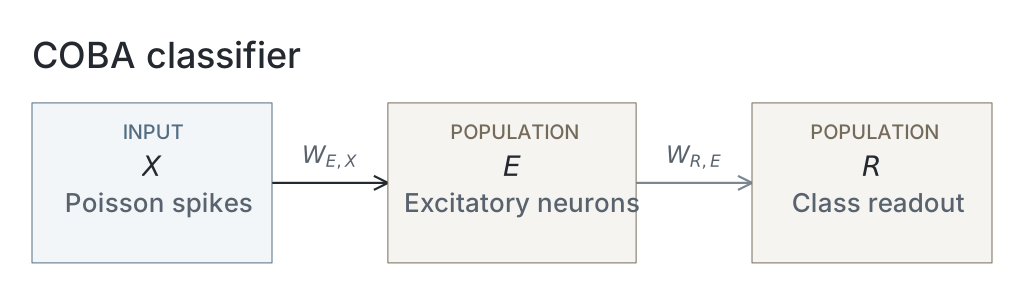
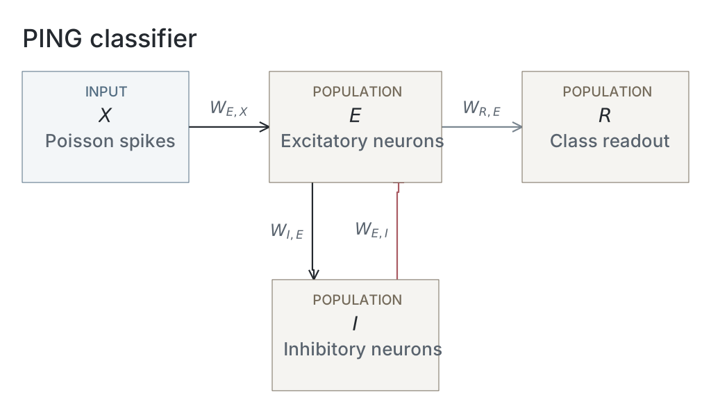
Parameters
Model values are read from original native snapshots through the selected presentation’s compute ancestry. Paired values are E / I. Initializer parent means and SDs describe the original weight distributions, in µS for conductance projections and dimensionless for the current-based readout; they are not measured trained-weight statistics. Missing snapshots or fields are unavailable; current recipes and historical copied tables are not substituted. The recorded configuration identifies the input, numerical and analysis choices of that computation; it does not establish a separate upstream training protocol.
| Parameter | COBA | PING |
|---|---|---|
| Network | ||
| E / I neurons | Unavailable / Unavailable | Unavailable / Unavailable |
| Output neurons | Unavailable | Unavailable |
| Neurons | ||
| Capacitance, E / I (nF) | Unavailable / Unavailable | Unavailable / Unavailable |
| Leak conductance, E / I (µS) | Unavailable / Unavailable | Unavailable / Unavailable |
| Resting voltage, E / I (mV) | Unavailable / Unavailable | Unavailable / Unavailable |
| Threshold, E / I (mV) | Unavailable / Unavailable | Unavailable / Unavailable |
| Reset, E / I (mV) | Unavailable / Unavailable | Unavailable / Unavailable |
| Refractory period, E / I | Unavailable / Unavailable | Unavailable / Unavailable |
| Synapses and weights | ||
| Input→E synapse | Unavailable / Unavailable | Unavailable / Unavailable |
| E→I synapse | Unavailable / Unavailable | Unavailable / Unavailable |
| I→E synapse | Unavailable / Unavailable | Unavailable / Unavailable |
| E→Output synapse | Unavailable / Unavailable | Unavailable / Unavailable |
| Input→E initializer parent mean / SD | Unavailable / Unavailable | Unavailable / Unavailable |
| E→I initializer parent mean / SD | Unavailable / Unavailable | Unavailable / Unavailable |
| I→E initializer parent mean / SD | Unavailable / Unavailable | Unavailable / Unavailable |
| E→Output initializer parent mean / SD | Unavailable / Unavailable | Unavailable / Unavailable |
| Native parameter stage | Unavailable | Unavailable |
| Input and simulation | ||
| Timestep (ms) | Unavailable | Unavailable |
| Duration (ms) | Unavailable | Unavailable |
| Evaluation samples | 1000 | 1000 |
| Seeds | Unavailable | Unavailable |
| Input rate (Hz) | Unavailable | Unavailable |
| Post-burn exclusion (ms) | Unavailable | Unavailable |
| Readout and training | ||
| Output neuron model | Unavailable | Unavailable |
| Epochs | Unavailable | Unavailable |
| Checkpoint role | final_epoch | final_epoch |
| Checkpoint purpose | endpoint_dynamics | endpoint_dynamics |
| Analysis | ||
| Frequency search (Hz) | Unavailable | Unavailable |
| Count-bin width (ms) | Unavailable | Unavailable |
| Autocorrelation maximum lag (ms) | Unavailable | Unavailable |
Dataset
Downstream: exp110 — Manuscript
Current runset
| Run | Date | Duration | Size | Evidence | Storage | Ran on | Verification |
|---|---|---|---|---|---|---|---|
| exp025-r014-present | 5s | 1.4 MB | Current | R2 | Local | Local: absent; R2: catalog-verified | |
| exp025-r013-analyse | 4s | 214.7 KB | Current | R2 | Local | Local: absent; R2: catalog-verified | |
| exp025-r009-analyse | 1m 4s | 205.4 KB | Current | R2 | HPC | Local: absent; R2: catalog-verified | |
| exp025-r008-compute | 1h 11m 46s | 33 MB | Current | R2 | HPC | Local: absent; R2: catalog-verified | |
| exp022-r015-compute | 12h 58m 52s | 3.6 GB | Current | R2 | HPC | Local: absent; R2: catalog-verified | |
| exp022-r007-compute | 11h 16m 8s | 3.6 GB | Current | R2 | HPC | Local: absent; R2: catalog-verified | |
| exp022-r001-compute | 2d 7h 4m 16s | 2 GB | Current | R2 | HPC | Local: absent; R2: catalog-verified |
References
- P. D. Welch. “The use of the fast Fourier transform for the estimation of power spectra: A method based on time averaging over short, modified periodograms.” IEEE Transactions on Audio and Electroacoustics 15(2), 70–73 (1967). doi:10.1109/TAU.1967.1161901.