Firing Rate Across the Timestep Sweep
Compares final-epoch firing rate, classification accuracy and illustrative rasters across a twelvefold integration-timestep sweep.
Abstract
We compared fifteen PING classifiers trained and evaluated at five matching integration timesteps from 0.05 to 0.6 ms, with fixed physical refractory periods and three seeds per condition. Test accuracy spanned 88.37–89.63%, while mean E firing ranged from 14.27 to 17.02 Hz. Timestep therefore affected these learned operating regimes. Because weights were trained separately, this tests complete training–evaluation pipelines rather than numerical convergence at fixed weights.
Results
Timestep rate and accuracy
Mean test accuracy ranged from 88.37% to 89.63%, spanning 1.27 percentage points. Mean E rate ranged from 14.27 to 17.02 Hz. Accuracy persisted across the tested resolutions, while firing remained timestep-dependent (Figure 1).

Figure 1: Hidden E rate (black) and test accuracy (red) across the twelvefold timestep sweep. Markers show means over 3 seeds; bars show ±1 standard error of the mean. Each network was evaluated on 1000 official-test images at its training timestep.
Timestep spike rasters
The same image produced distinct E/I spike patterns across the separately trained timesteps. These single-seed illustrations do not establish invariance of the gamma period.

Figure 2: E (black) and I (red) rasters for the same official-test image, seed 42, at timesteps (A–E) 0.05, 0.1, 0.2, 0.3 and 0.6 ms, respectively. Panels display 200 E and 64 I neurons over the first 100 ms. These illustrative probes support visual cadence inspection, not a population estimate of gamma-period invariance.
Training-timestep response
The endpoint E-rate differences above persisted after the same finite training horizon. Validation trajectories show each network separately; they do not establish an asymptotic firing-rate ceiling.

Figure 3: Recorded training histories: (A) validation accuracy and (B) E rate, one line per timestep and seed. Each epoch averaged 3 encoder draws per validation image. The final-epoch comparison is a finite-training snapshot, not an established fixed-point ceiling.
Methods
The audit reused separately trained networks and their learning histories, then measured endpoint dynamics at matched training and inference timesteps.
-
Reuse the trained population. One PING network was trained per ms and seed , giving fifteen networks. Each had 784 inputs, 1024 excitatory neurons, 256 inhibitory neurons and 10 class outputs. Network geometry, synaptic settings, readout and optimisation settings were checked for agreement across the comparison. E/I refractory holds were fixed at 1.2/0.6 ms: 24/12, 12/6, 6/3, 4/2 and 2/1 steps, respectively. Twelve networks were newly trained for this design; three 0.1-ms networks were reused unchanged after execution-equivalence checks.
-
Keep data and nominal duration fixed. The 7000-image MNIST training pool contained 6300 optimisation images and 700 validation images; the official test partition was excluded from training. The nominal presentation duration was 200 ms; whole-step rounding gave 4,000, 2,000, 1,000, 666 and 333 steps. Realised was 199.8 ms at 0.3/0.6 ms and 200 ms otherwise. Image intensities drove Poisson input with peak rate 25 Hz.
-
Use the training endpoint. Networks underwent 50 epochs of surrogate-gradient training [1], with batch size 256 and learning rate 0.0004. Class scores used the mean-membrane readout, and validation histories averaged 3 encoder draws per image. The audit used the final epoch for rates, accuracy and rasters, rather than selecting the best validation epoch.
-
Measure held-out performance. Each network was evaluated on the fixed 1000-image subset of the official MNIST test partition, without retraining. Accuracy was the percentage of correctly classified images; population firing rate was total spikes divided by the number of evaluated images, population size and realised trial duration in seconds. Excitatory and inhibitory rates were recorded separately.
Network diagrams
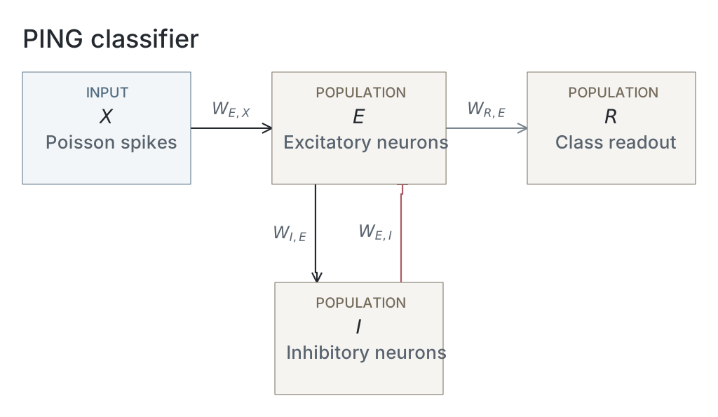
Parameters
Model values are read from original native snapshots through the selected presentation’s compute ancestry. Paired values are E / I. Initializer parent means and SDs describe the original weight distributions, in µS for conductance projections and dimensionless for the current-based readout; they are not measured trained-weight statistics. Missing snapshots or fields are unavailable; current recipes and historical copied tables are not substituted. The recorded configuration identifies the input, numerical and analysis choices of that computation; it does not establish a separate upstream training protocol.
| Parameter | PING |
|---|---|
| Network | |
| E / I neurons | Unavailable / Unavailable |
| Output neurons | Unavailable |
| Neurons | |
| Capacitance, E / I (nF) | Unavailable / Unavailable |
| Leak conductance, E / I (µS) | Unavailable / Unavailable |
| Resting voltage, E / I (mV) | Unavailable / Unavailable |
| Threshold, E / I (mV) | Unavailable / Unavailable |
| Reset, E / I (mV) | Unavailable / Unavailable |
| Refractory period, E / I | Unavailable / Unavailable |
| Synapses and weights | |
| Input→E synapse | Unavailable / Unavailable |
| E→I synapse | Unavailable / Unavailable |
| I→E synapse | Unavailable / Unavailable |
| E→Output synapse | Unavailable / Unavailable |
| Input→E initializer parent mean / SD | Unavailable / Unavailable |
| E→I initializer parent mean / SD | Unavailable / Unavailable |
| I→E initializer parent mean / SD | Unavailable / Unavailable |
| E→Output initializer parent mean / SD | Unavailable / Unavailable |
| Native parameter stage | Unavailable |
| Input and simulation | |
| Timestep (ms) | Unavailable |
| Duration (ms) | 200 |
| Evaluation samples | 1000 |
| Seeds | 42 / 43 / 44 |
| Input rate (Hz) | Unavailable |
| Post-burn exclusion (ms) | Unavailable |
| Readout and training | |
| Output neuron model | Unavailable |
| Epochs | Unavailable |
| Checkpoint role | final_epoch |
| Checkpoint purpose | endpoint_dynamics |
| Analysis | |
| Frequency search (Hz) | Unavailable |
| Count-bin width (ms) | Unavailable |
| Autocorrelation maximum lag (ms) | Unavailable |
Dataset
Downstream: exp110 — Manuscript
Current runset
| Run | Date | Duration | Size | Evidence | Storage | Ran on | Verification |
|---|---|---|---|---|---|---|---|
| exp044-r009-present | 2s | 376.4 KB | Current | R2 | Local | Local: absent; R2: catalog-verified | |
| exp044-r008-analyse | 3s | 152.8 KB | Current | R2 | Local | Local: absent; R2: catalog-verified | |
| exp044-r007-compute | 2m 25s | 112.7 KB | Current | R2 | Local | Local: absent; R2: catalog-verified | |
| exp022-r007-compute | 11h 16m 8s | 3.6 GB | Current | R2 | HPC | Local: absent; R2: catalog-verified | |
| exp022-r001-compute | 2d 7h 4m 16s | 2 GB | Current | R2 | HPC | Local: absent; R2: catalog-verified |
References
- E. O. Neftci, H. Mostafa, and F. Zenke. “Surrogate Gradient Learning in Spiking Neural Networks.” IEEE Signal Processing Magazine 36(6), 51–63 (2019). doi:10.1109/MSP.2019.2931595