One Spike per Gamma Cycle
Pooled and equally weighted network distributions support predominantly one-spike gamma-cycle participation across 18 trained networks, with exceptions.
Abstract
We measured excitatory spikes per inhibitory-burst cycle in eighteen trained PING networks, comparing opportunity pooling with equal-network averaging across six decay conditions. The equal-network mean assigned 76.35% of neuron–cycle pairs to silence and 22.09% to one spike. Single-spike participation predominated among active pairs, but repeated spikes and above-reference firing rates preclude a strict one-spike ceiling. These measurements do not establish a universal participation law.
Results
Spikes per neuron-cycle
Across the balanced 18-network design, the equal-network mean assigned 76.35% of pairs to zero spikes, 22.09% to one spike and 1.56% to two or more spikes. Thus, 98.44% contained at most one spike (Fig. 1).

Figure 1: Equal-network distributions of excitatory spikes per neuron–cycle at values (A–F) 4.5, 6, 9, 12, 18 and 27 ms. Each separately trained network’s counts of pairs with 0, 1, 2 or ≥3 spikes were normalized to sum to one; black bars are arithmetic means across the three networks per condition, irrespective of their detected cycle totals. These distributions reuse epoch-50 spike recordings from the inhibitory-timescale sweep. Presentations without detected inhibitory bursts are excluded; no uncertainty interval is shown.
For comparison, opportunity pooling across 167,178,240 neuron–cycle pairs assigned 75.24% of pairs to zero spikes and 23.62% to one spike. Two-or-more events occurred in 1.15% of pairs and three-or-more in 0.10%; pooled over the sweep, 98.85% contained at most one spike. Among active pairs, 95.37% contained exactly one spike, declining from 98.93% at 4.5-ms inhibitory decay to 83.78% at 27 ms. Single-spike participation predominated, but its frequency depended on the decay condition.
Giving each trained network equal weight within its decay condition changed each spike-count fraction by less than 0.20 percentage points relative to opportunity pooling; the largest shift was 0.191 percentage points in the one-spike fraction at ms. Pooling samples a neuron–cycle pair uniformly, whereas equal-network averaging first samples a network uniformly. The latter also balances the six decay conditions; pooling gives more weight to the faster rhythms that produced more cycles.
Rate versus gamma frequency
Maximum per-neuron excitatory firing rate, , scaled with spectral-peak frequency, , with through-origin fit and coefficient of determination (Fig. 2). Both rates are in hertz. Four of the 18 network maxima exceeded the one-spike-per-cycle reference, including 80.97 Hz at 67.21 Hz. Proximity of the fitted slope to one therefore does not establish a strict ceiling.

Figure 2: Per-neuron E rate versus measured gamma frequency across the sweep. Triangles and circles show each network’s maximum and median neuron rates, respectively, averaged over all test presentations; colours group decay conditions. The dashed line is , where is per-neuron E rate. The dotted line is a fixed visual reference, not a fitted participation estimate. Neither line is the fitted maximum-rate model.
Methods
We reused spike recordings from the epoch-50 checkpoints of the inhibitory-timescale sweep: six decay conditions and three independently trained networks per condition (seeds 42–44). The equal-network comparison reanalysed these recordings without retraining or new inference.
-
Evaluate fixed test presentations. The reused evaluation presented the same fixed 1,000-image subset of the official MNIST test partition to each network for 200 ms per image, with a 0.1-ms timestep. Recordings contained spikes from all 1,024 excitatory and 256 inhibitory neurons and mean per-neuron excitatory firing rates over the complete evaluation.
-
Detect inhibitory bursts. We smoothed inhibitory population spike counts with a unit-sum Gaussian of 1-ms standard deviation, extending ±4 ms. Peaks reached at least 5% of each presentation’s maximum smoothed count and were separated by at least half the network’s spectral period, rounded down to simulation steps. We reused , the interpolated 5–150-Hz peak of each network’s trial-averaged excitatory Welch spectrum.
-
Define cycles. Boundaries were integer midpoints between consecutive inhibitory peaks, rounded down; edge intervals extended to presentation boundaries and could contain partial cycles. A single burst defined one full-presentation interval. Presentations without detected bursts were excluded from cycle counts, but not whole-presentation firing rates.
-
Count excitatory spikes. We counted each neuron’s spikes separately in each interval, including its starting step and excluding its ending step. Inhibitory bursts supplied the cycle anchor even when an excitatory neuron remained silent.
-
Estimate opportunity and network distributions. We bucketed spike counts into . For the opportunity-pooled distribution, we summed bucket counts across neurons, cycles and networks before normalization. For the equal-network distribution, we normalized each network’s bucket counts separately and then took their arithmetic mean, giving the three networks equal weight within each condition and all 18 networks equal weight in the across-sweep summary. A network with no detected cycles would have an undefined distribution and abort this analysis; none did. Active-pair fractions excluded zero-spike pairs. Neurons and cycles were not independent training replicates; no uncertainty interval was estimated for the network distributions.
-
Compare rates and frequency. We fitted maximum per-neuron E rate against by least squares through the origin across all 18 networks, weighting networks equally. The reported used the centred total sum of squares. Median-neuron rates and the fixed reference lines were displayed separately from this fit.
Network diagrams
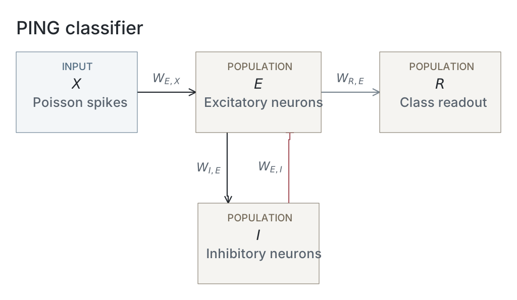
Parameters
Model values are read from original native snapshots through the selected presentation’s compute ancestry. Paired values are E / I. Initializer parent means and SDs describe the original weight distributions, in µS for conductance projections and dimensionless for the current-based readout; they are not measured trained-weight statistics. Missing snapshots or fields are unavailable; current recipes and historical copied tables are not substituted. The recorded configuration identifies the input, numerical and analysis choices of that computation; it does not establish a separate upstream training protocol.
| Parameter | PING |
|---|---|
| Network | |
| E / I neurons | Unavailable / Unavailable |
| Output neurons | Unavailable |
| Neurons | |
| Capacitance, E / I (nF) | Unavailable / Unavailable |
| Leak conductance, E / I (µS) | Unavailable / Unavailable |
| Resting voltage, E / I (mV) | Unavailable / Unavailable |
| Threshold, E / I (mV) | Unavailable / Unavailable |
| Reset, E / I (mV) | Unavailable / Unavailable |
| Refractory period, E / I | Unavailable / Unavailable |
| Synapses and weights | |
| Input→E synapse | Unavailable / Unavailable |
| E→I synapse | Unavailable / Unavailable |
| I→E synapse | Unavailable / Unavailable |
| E→Output synapse | Unavailable / Unavailable |
| Input→E initializer parent mean / SD | Unavailable / Unavailable |
| E→I initializer parent mean / SD | Unavailable / Unavailable |
| I→E initializer parent mean / SD | Unavailable / Unavailable |
| E→Output initializer parent mean / SD | Unavailable / Unavailable |
| Native parameter stage | Unavailable |
| Input and simulation | |
| Timestep (ms) | Unavailable |
| Duration (ms) | Unavailable |
| Evaluation samples | 1000 |
| Seeds | 42 / 43 / 44 |
| Input rate (Hz) | Unavailable |
| Post-burn exclusion (ms) | Unavailable |
| Readout and training | |
| Output neuron model | Unavailable |
| Epochs | Unavailable |
| Checkpoint role | final_epoch |
| Checkpoint purpose | endpoint_dynamics |
| Analysis | |
| Frequency search (Hz) | Unavailable |
| Count-bin width (ms) | Unavailable |
| Autocorrelation maximum lag (ms) | Unavailable |
Dataset
Upstream: exp022 — MNIST, exp041 — Firing Rate Tracks Gamma Frequency
Downstream: exp110 — Manuscript
Current runset
| Run | Date | Duration | Size | Evidence | Storage | Ran on | Verification |
|---|---|---|---|---|---|---|---|
| exp046-r010-present | 2s | 718.6 KB | Current | R2 | Local | Local: absent; R2: catalog-verified | |
| exp046-r007-analyse | 25s | 465.9 KB | Current | R2 | Local | Local: absent; R2: catalog-verified | |
| exp046-r001-compute | — | 101.5 MB | Current | R2 | Unknown | Local: absent; R2: catalog-verified | |
| exp041-r002-analyse | 3s | 1.8 MB | Current | R2 | Local | Local: absent; R2: catalog-verified | |
| exp041-r001-compute | — | 7.7 MB | Current | R2 | Unknown | Local: absent; R2: catalog-verified | |
| exp022-r001-compute | 2d 7h 4m 16s | 2 GB | Current | R2 | HPC | Local: absent; R2: catalog-verified |