Pool Size and Synaptic Scaling

Abstract

We tested inhibitory pool size under two controls: fixed summed inhibition and fixed expected per-synapse strength. Across 3 seeds, increasing I size from 16 to 256 changed mean E firing from 6.01 to 6 Hz at fixed summed coupling, versus 16.62 to 6 Hz at fixed synaptic strength. Pool-size effects depended on scaling. These untrained-network rates do not by themselves establish gamma oscillations.

Results

Pool-size scaling response

At nominal $G_{I \to E} =$ 2 μS, E rates changed from 6.01 to 6 Hz across 16–256 I neurons. At $\bar{w}_{I \to E} \approx$ 7.81 nS, E rates fell from 16.62 to 6 Hz and I rates from 120.41 to 34.41 Hz. All tested fixed-mean levels showed this decrease, consistent with stronger summed inhibition and reduced E–I feedback (Fig. 1).

Methods

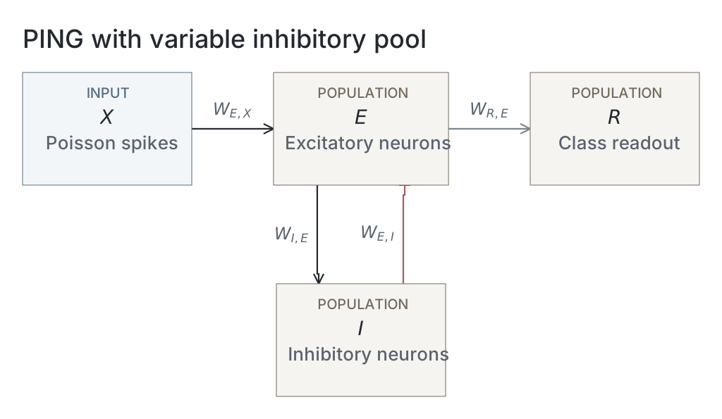
We compared two scaling controls using recorded outputs from simulations of untrained, dense recurrent excitatory–inhibitory networks, without additional simulation.

1. Initialize fan-in-normalized weights. For an I→E matrix with 1024 excitatory columns and $N_{I}$ inhibitory rows, each weight was $W_{k j}^{I E} = \frac{G_{\text{draw}}}{N_{I}}$, with $G_{\text{draw}} = \max ( 0 , X )$ and $X \sim \mathcal{N} ( \mu_{\text{init}} , \sigma_{\text{init}}^{2} )$ a Gaussian draw of mean $\mu_{\text{init}}$ and standard deviation $\sigma_{\text{init}} = 0.1 \mu_{\text{init}}$, in μS. Defining expected summed coupling $G_{I \to E} = \mathcal{E} [ G_{\text{draw}} ]$ gives

   $$\mathcal{E} [ W_{k j}^{I E} ] = \bar{w}_{I \to E} = \frac{G_{I \to E}}{N_{I}} , \quad \mathcal{E} [ \sum_{k = 1}^{N_{I}} W_{k j}^{I E} ] = G_{I \to E} . \tag{1}$$

   Here $\mathcal{E}$ averages over weight initialization, $k$ indexes inhibitory neurons and $j$ excitatory neurons; $\bar{w}_{I \to E}$ is the expected conductance of one synapse, not an identical realised weight. An inhibitory volley gives

   $$\Delta g_{\text{inh,post=E} , j} = \sum_{k \in \mathcal{I}_{\text{active}}} W_{k j}^{I E} , \tag{2}$$

   where $\mathcal{I}_{\text{active}}$ is the active inhibitory set and $\Delta g_{\text{inh,post=E} , j}$ the inhibitory conductance increment at E neuron $j$, in μS; both weights and participation therefore enter the increment.

2. Apply paired pool-size controls. We swept $N_{I} \in \{$16, 64, 256$\}$. Fixed-summed controls used parent means $\mu_{\text{init}} \in \{$1, 2, 4$\}$ μS, so $\bar{w}_{I \to E} \propto \frac{1}{N_{I}}$; fixed-mean-synapse controls scaled $\mu_{\text{init}}$ with $N_{I}$, giving nominal $\bar{w}_{I \to E} \in \{$3.90625, 7.8125, 15.625$\}$ nS. Nominal values approximate the post-clamp expectations; the arms coincide at 256 I neurons, with one additional shared condition at 64 I neurons and nominal 1 μS summed coupling.

3. Drive and measure the networks. Nominal E→I summed coupling stayed at 1 μS; input weights used parent mean 1.2 μS, 95% initial zeros, compensation for zeroing and fan-in normalization. Each network received 784 independent 25 Hz input channels, implemented as Bernoulli spikes per 0.1 ms timestep, for 500 ms and 8 trials, with seeds 40, 41, 42. We included all conditions and averaged spike counts over the full duration, trials and neurons within each population; overlapping controls reused measurements, giving 3 seeds at each of 18 conditions from 42 distinct simulations. The reanalysis used these rates, not raw spike trains; population rates alone do not establish gamma oscillations [1].

4. Display pool-size comparisons. We displayed the recorded population-rate responses for fixed total and fixed per-synapse coupling with their shared controls and seed aggregation.

References

- G. Buzsáki and X.-J. Wang. “Mechanisms of Gamma Oscillations.” Annual Review of Neuroscience 35, 203–225 (2012). doi:10.1146/annurev-neuro-062111-150444