Mean-Field Analysis of PING Bifurcations
An independent four-variable mean-field analysis identifies a Hopf bifurcation, sampled dynamics consistent with a supercritical transition, and decreasing onset frequency with slower inhibition.
Abstract
We analysed the four-state E→I→E specialisation of the mean-field model. Analytical-Jacobian continuation identified a Hopf bifurcation at 0.593905 nA with onset frequency 27.57 Hz. Ascending and descending near-onset integrations produced coincident sampled branches and continuous amplitude growth consistent with a supercritical transition. This numerical criterion does not exclude a narrower bistable interval or unstable cycle. Hopf frequency decreased as inhibitory decay lengthened.
Results
A reversible Hopf onset slows
At 0.593905 nA, a complex-conjugate eigenvalue pair crossed the imaginary axis at 27.57 Hz (Fig. 1A). The sampled amplitude branches differed by at most 0.00687 Hz and had 0.9994, consistent with a supercritical transition (Fig. 1B). Across the inhibitory-decay sweep, decreased from 30.2 to 17.94 Hz (Fig. 1C). Finite spacing cannot exclude narrower bistability or an unstable periodic orbit.

Mean-field Hopf bifurcation. (A) All four eigenvalues, coloured by external drive; open markers identify the refined Hopf pair. (B) Peak-to-peak excitatory-rate amplitude over the final 500 ms of each ascending or descending drive condition, relative to the refined Hopf drive. (C) Refined Hopf frequency at and ms, with all other model parameters fixed. These deterministic calculations have no statistical uncertainty intervals.
Methods
The selected results precede the SNNLab 0.27 migration. They retain their original solver settings; the current recipe has not regenerated these displayed results.
-
Model. The mean-field note supplies the shared derivation; Appendix A records this experiment’s specialisation.
-
Hopf bifurcation and onset frequency. At the reference inhibitory-pathway decay ms, we evaluated the equilibrium over 401 equally spaced external drives from 0 to 4 nA.
2.1 — Solve for the equilibrium.
Set the two recurrent conductance derivatives to zero in the note’s equations, apply the experimental specialisation, and substitute the inhibitory equilibrium rate into the excitatory equation. The scalar residual is the excitatory rate minus its predicted gain.
Brent’s bracketed method searched with absolute tolerance and relative tolerance . We recovered , and by substitution and required an absolute residual below .
2.2 — Calculate local stability. At every equilibrium, we evaluated the analytical reduced Jacobian and numerically calculated its four eigenvalues. Eigenvalues with positive imaginary part greater than were eligible for the leading complex pair. We plotted all four eigenvalues in the complex plane and coloured them by external drive; negative and positive real parts denoted local decay and growth, respectively (Fig. 1A).
2.3 — Identify and verify the crossing.
The first change of the leading complex pair from negative to nonnegative real part supplied a coarse drive bracket. Brent’s method refined the zero to absolute drive tolerance nA and relative tolerance , recomputing the equilibrium and analytical Jacobian at every trial drive. We confirmed nonzero imaginary part, negative real parts for the remaining modes, and positive transversality by a centred difference with nA half-step. The recorded crossing slope was 0.29 and the largest remaining real part was -0.458 .
2.4 — Calculate the onset frequency. At the refined crossing, was the magnitude of the critical pair’s imaginary part in radians per millisecond. We converted it to hertz using (Fig. 1A).
-
Numerical criticality test. We integrated 25 equally spaced drives from 0.1 nA below to 0.55 nA above the refined Hopf point, first in ascending and then in descending order. The initial state was the lowest-drive equilibrium with an added excitatory-rate perturbation; each subsequent condition began from the preceding endpoint. LSODA integrated each condition for 2,000 ms with relative tolerance , absolute tolerance and maximum step 1 ms.
For each drive, peak-to-peak excitatory-rate amplitude was measured over the final 500 ms. We classified the sampled dynamics as consistent with a supercritical transition when the maximum difference between ascending and descending amplitudes was below , and ordinary least-squares regression of on above onset had positive slope and . This finite numerical criterion tests reversible, continuous onset; it does not detect an unstable cycle or prove the absence of narrower bistability.[1]
-
Inhibitory-decay sweep. We repeated the equilibrium continuation and refined complex-pair crossing at and ms while holding all other model parameters fixed. At every decay constant, we applied the same nonzero-frequency, remaining-mode stability and transversality checks used at the 6-ms reference condition, then converted the critical angular frequency to in hertz.
Appendix A — Model specialisation and stability
A1 — Experimental specialisation
The mean-field note defines the model and its derivation. This experiment disables E→E and I→I coupling and has no external conductance input. Instead, is the swept tonic current and . The four-state reduction therefore uses .
Rates are spikes per neuron per ms. The decay times are ms and swept ; the resting-voltage driving forces are mV and mV for both populations . The fixed noise scale is mV; rate-relaxation times are 20/5 ms for E/I. Recorded values and numerical settings are listed in the parameter table.
The note’s matrix sums denote this experiment’s imported reference couplings, not newly sampled matrices. The tonic current is a control parameter; no empirical input-rate mapping is inferred. The general gain, fixed-driving-force approximation and rate relaxation are not rederived here.
A2 — Stability calculation
The zero-self-coupling Jacobian applies directly with the experimental parameters above. The note gives the analytical gain slope and stability criteria. The numerical continuation, crossing checks and criticality test remain in Methods.
Setting the conductance and rate derivatives to zero defines the stationary problem in Method 2.1. Native SNNLab calculations solve all four equations together; the earlier calculation used scalar elimination.
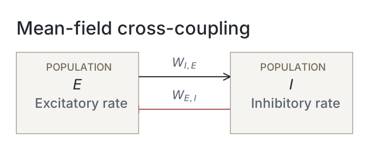
Network diagrams
Parameters
This is an analytical population calculation, so simulation snapshots do not apply. Native runs export the SNNLab model document, including equations, parameters and closure assumptions. Imported constants and numerical choices below come from the selected computation’s recorded configuration. Missing historical fields are unavailable; current defaults are never substituted.
| Parameter | Recorded value |
|---|---|
| Network: imported reference sizes | |
| E / I neurons | 1024 / 256 |
| Neurons: imported reference physics | |
| Capacitance, E / I (nF) | 1 / 0.5 |
| Leak conductance, E / I (µS) | 0.05 / 0.1 |
| Membrane time constant, E / I (ms; capacitance / leak) | 20 / 5 |
| Rest / reset / threshold (mV) | -65 / -65 / -50 |
| Excitatory / inhibitory reversal (mV) | 0 / -80 |
| Refractory period, E / I (ms) | 1.2 / 0.6 |
| Synapses: imported reference coupling | |
| AMPA / reference GABA decay (ms) | 2 / 6 |
| E→I / I→E summed coupling (µS) | 1 / 2 |
| Closure assumptions and experimental choices | |
| Rate relaxation, E / I (ms) | 20 / 5 |
| Effective voltage noise (mV) | 4 |
| Driving-force reference | resting_voltage |
| External drive minimum / maximum (nA) | 0 / 4 |
| GABA-decay sweep (ms) | 4.5 / 6 / 9 / 12 / 18 / 27 |
| Numerical analysis | |
| Drive-grid minimum / maximum (nA) / point count | 0 / 4 / 401 |
| Equilibrium solver | brentq |
| Native scaled derivative tolerance | Unavailable |
| Gain quadrature nodes | Unavailable |
| Historical equilibrium absolute / relative tolerances | 1e-13 / 1e-12 |
| Equilibrium residual tolerance (per ms) | 1e-11 |
| Complex-pair imaginary threshold (per ms) | 1e-8 |
| Hopf solver / absolute tolerance (nA) | brentq / 1e-12 |
| Hopf relative tolerance / transversality step (nA) | 1e-12 / 0.00001 |
| Ramp relative-drive endpoints (nA) | -0.1 / 0.55 |
| Ramp points / duration (ms) | 25 / 2000 |
| Ramp measurement start (ms) / samples | 1500 / 1001 |
| Initial E-rate perturbation (per ms) | 0.001 |
| Amplitude / branch-gap thresholds (per ms) | 0.0001 / 0.0001 |
| Minimum amplitude-squared fit R² | 0.9 |
| Ramp solver | LSODA |
| Ramp relative / absolute tolerances | 1e-7 / 1e-10 |
| Maximum integration step (ms) | 1 |
Dataset
Upstream: —
Downstream: exp110 — Manuscript
Current runset
| Run | Date | Duration | Size | Evidence | Storage | Ran on | Verification |
|---|---|---|---|---|---|---|---|
| exp117-r025-present | <1s | 323.4 KB | Current | R2 | Local | Local: absent; R2: catalog-verified | |
| exp117-r024-analyse | <1s | 265 KB | Current | R2 | Local | Local: absent; R2: catalog-verified | |
| exp117-r023-compute | 30s | 1.6 MB | Current | R2 | Local | Local: absent; R2: catalog-verified |
References
- Y. A. Kuznetsov. Elements of Applied Bifurcation Theory, third edition. Springer (2004), Chapters 3 and 5. doi:10.1007/978-1-4757-3978-7