Decision Time and Gamma Cycles
Paired inhibitory-decay probes of output evidence, sustained decisions and network spike cost at a 25 Hz input encoding rate.
Abstract
We examined how inhibitory decay changes activity and decision-making in a trained spiking network. Longer decay slowed the network’s rhythm and reduced its spike rate. Across a shared image sample, longer decay generally delayed correct decisions and reduced spike consumption, while lowering accuracy at a fixed deadline. Decision timing varied by image, and comparisons at later completed-volley counts depended on trial coverage. These results show a trade-off in one trained network: reaching 80% accuracy took 38 ms and 5,135 mean network spikes at 3 ms decay, versus 144 ms and 3,706 spikes at 30 ms.
Background
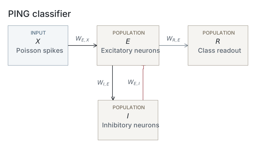
We imported the trained PING network from exp022 — MNIST and kept its weights fixed. The parameter table lists the network and simulation settings.
Results
Inhibitory decay and network dynamics
We tested one trained network on 500 MNIST test images, 50 per digit, with ten random spike encodings per image. We reused each encoding at 19 inhibitory decay settings, , from 3 to 30 ms. Each presentation lasted 200 ms, with network state reset between presentations. All five figures use this shared sweep of 95,000 presentations. Sampling seeds, encoding rates and simulation settings are listed in the parameter table. No uncertainty estimates are shown.
Longer inhibitory decay slowed the rhythm and reduced firing (Figure 1, A and C). From 3 to 30 ms decay, the spectral peak fell from 100.2 to 17.7 Hz and excitatory firing fell from 26,589 to 5,377 spikes/s. The fraction of excitatory neurons active per accepted cycle stayed between 20.9% and 24.5% (B). Spectral peaks can select harmonics; these results come from one trained network.

A–D show rhythm frequency, the percentage of excitatory neurons active per cycle, total excitatory spikes per second, and rhythm contrast. Results use 500 images and ten encodings per image at each decay setting. Frequency is the peak of the mean excitatory power spectrum; contrast measures the height of an autocorrelation peak above its neighbouring trough. Participation uses accepted complete cycles only. Dashed lines mark the 6 ms training setting. E–G show image 0, draw 42, at 3, 6 and 12 ms decay: excitatory spikes are black and inhibitory spikes red. All measurements cover 200 ms.
Evidence across time
Higher-frequency groups generally developed high correct-digit scores sooner (Figure 2). The pattern varied by image; image 115 (F) kept much lower scores than most examples.

Each panel shows one example image. Each line shows the correct digit’s mean softmax score across ten encodings at one decay setting. Darker colours mean higher I-volley frequency, averaged across accepted trials over the full 200 ms. Frequency is the reciprocal of the mean interval between inhibitory volleys. The colour scale is shared with Figure 3. Scores are sampled every 1 ms; they are not accuracy or calibrated probabilities.
The nine examples are the first selected image indices: 0, 7, 29, 51, 71, 115, 140, 161 and 164. For digit , counts its output spikes by time :
Here, is elapsed time, is the timestep, indexes simulation steps, and is one when output neuron spikes, otherwise zero. We converted these logits into scores using softmax:
Here, is the score for digit , and ranges over all ten digits. We applied softmax before averaging the correct digit’s score across ten encodings. All scores start at 0.1. The network was trained using mean voltage; this spike-count readout was not retrained or calibrated.
Evidence per completed volley
Several images reached high scores within a few completed volleys (Figure 3). The traces do not align exactly: early scores vary with decay, image 115 remains distinct, and later counts use different trial subsets. Score saturation can also make traces look aligned.

The same images, scores and colours as Figure 2, plotted against completed inhibitory volleys. Dots mark the trough between successive volleys; lines join integer counts. Each score averages available accepted trials and requires at least eight of ten encodings. Later counts can therefore include different trials. Count zero is the initial score of 0.1; the final volley is excluded if it has no following trough.
We detected inhibitory volleys after 1 ms Gaussian smoothing, requiring peaks at least 2 ms apart and prominence of at least one spike or 20% of the maximum, whichever was larger. Accepted sequences needed a complete interior cycle and at least 50% mean inhibitory participation. A volley ended at the trough between its peak and the next; we sampled the accumulated output score there. We did not extend traces beyond the last bounded completion.
Sustained correct decisions
Higher frequencies generally accompanied shorter decision times, while median volley counts stayed near one or two over much of the range (Figure 4). Decisions before the first trough count as one; this does not mean a whole volley was necessary. These plots include only eligible successful trials. Frequency uses the full 200 ms, including activity after the decision, so the association does not show that frequency alone sets classification speed.

A: time to a lasting correct decision. B: the first completed-volley count at or after that decision. Both are plotted against each trial’s I-volley frequency. Cells span 5 ms × 5 Hz in A and one volley × 5 Hz in B. Darker cells contain more trials on a logarithmic scale; white cells are empty. Black lines show medians within 5 Hz bands. From 95,000 presentations, A includes 84,237 trials and B includes 80,341, using the rules below.
A lasting correct decision is the first update after which the correct digit stays the unique output-spike-count winner through 200 ms. Ties break stability. This looks back over the full trial; it is not an online stopping rule.
Of 95,000 trials, 84,284 had a lasting correct decision. Of these, 84,237 also had an accepted frequency and appear in A. Panel B also requires a decision no later than the final bounded completion and at least eight of ten encodings with enough completed volleys at that count, leaving 80,341 trials.
Spike cost at 80% accuracy
Slower settings saved spikes at the cost of time (Figure 5). At 3 ms decay, reaching 80% accuracy took 38 ms and 5,135 mean network spikes. At 30 ms decay, it took 144 ms and 3,706 spikes: 28% fewer spikes, but 3.8 times longer. Mean I-volley frequencies were about 107 and 15 Hz.

Time and mean network spikes needed to first reach 80% accuracy, checked every 1 ms. Both measurements use all 500 images and ten encodings per image, including incorrect predictions. Spikes include excitatory, inhibitory and output neurons, but exclude input. Circles show 14 of the 19 decay settings: each offers a speed–cost choice that no other setting improves on both measures. Lines join measured points only. Darker colours mean higher mean I-volley frequency over 200 ms. The second colour bar shows the corresponding decay settings; its spacing follows their measured frequencies.
For each setting, predictions used the largest accumulated output spike count; the lowest digit won ties. All 19 settings reached 80%. Unlike Figure 4, accuracy could fall again after crossing the target. The 80% target was chosen for this exploratory comparison, and the curve was selected on the same test sample. Costs are averages, not individual stopping costs or physical energy. Other accuracy targets can give different curves.
Network diagrams
Parameters
| Parameter | Recorded value |
|---|---|
| Network | |
| Native parameter snapshot | Unavailable |
| Input channels | Unavailable |
| Populations | Unavailable |
| Membrane model | Unavailable |
| Neurons | |
| Membrane capacitance | Unavailable |
| Leak conductance | Unavailable |
| Resting potential | Unavailable |
| Reset potential | Unavailable |
| Threshold | Unavailable |
| Refractory period | Unavailable |
| Membrane time constant | Unavailable |
| Synapses and weights | |
| Native synapse and weight parameters | Unavailable |
| Input and simulation | |
| Partition | official_mnist_test |
| Image selection | 50 randomly sampled per digit without replacement |
| Selection seed | 123 |
| Test images | 500 |
| Encoding identifiers | [42,43,44,45,46,47,48,49,50,51] |
| Inhibitory decay settings | [3,3.367386144928119,3.77976314968462,4.242640687119285,4.762203155904599,5.345392308842037,6,6.734772289856239,7.559526299369239,8.485281374238571,9.524406311809198,10.690784617684075,12,13.979916609008557,16.28650569956944,18.973665961010276,22.104188991842317,25.75122656797671,30] ms |
| Input rates | [25] Hz |
| Generator seed rule | 1000 * image_index + encoding_seed |
| Timestep | 0.1 ms |
| Duration | 200 ms |
| Burn-in | 0 ms |
| Checkpoint role | final_epoch |
| Checkpoint SHA-256 | 34a94d90e652059ef754a214670d2fe642af504a6fcc01380d33bd22854278c6 |
| Analysis | |
| schema | exp123.measurement/v1 |
| score | softmax of cumulative output spike counts |
| softmax temperature | 1 |
| time sampling | zero state plus each completed integration step |
| primary score | true class |
| volley smoothing ms | 1 |
| volley spacing ms | 2 |
| volley relative prominence | 0.2 |
| volley minimum prominence | 1 |
| minimum i participation pct | 50 |
| phase origin | first detected I volley = zero |
| phase interpolation | linear between successive volley times; no extrapolation |
| phase grid step | 0.05 |
| volley count origin | first accepted I volley = one; each subsequent accepted volley increments count |
| volley scores | sample cumulative scores at the first minimum of smoothed I activity strictly between each accepted peak and the next; last completed update; final peak has no completion |
| completed volley count origin | one at the trough following the first accepted I peak; zero is illustrative time-zero state |
| decision volley count | number of accepted I volleys at or before decision; accepted coverage only |
| decision completed volley count | first inhibitory trough completion at or after stable decision; one-based; accepted sequences and shared Figure 2 count range only; decisions after last bounded completion excluded |
| phase coverage | within each decay setting, available accepted draws only; display completed-volley scores at >=80% draw coverage; no extrapolation |
| saturation threshold | 0.99 |
| decision rule | earliest unique true-class cumulative-count winner sustained through the final update; ties are failures |
| decision cycle mapping | interpolate within each accepted I-volley sequence only; no extrapolation |
| decision summary | median and quartiles among successful trials; cycle summaries require an in-range accepted cycle coordinate |
| decision completed volley coverage | accepted sequence, in-range completion and >=80% draw coverage at that count within its decay setting |
Dataset
Downstream: exp134 — PING: Leak and Capacitance
Current runset
| Run | Date | Duration | Size | Evidence | Storage | Ran on | Verification |
|---|---|---|---|---|---|---|---|
| exp123-r079-present | 3s | 22.7 MB | Current | R2 | Local | Local: absent; R2: catalog-verified | |
| exp123-r078-analyse | 28m 51s | 42.8 MB | Current | R2 | Local | Local: absent; R2: catalog-verified | |
| exp123-r068-compute | 1h 16m 39s | 961.4 MB | Current | R2 | Local | Local: absent; R2: catalog-verified | |
| exp022-r001-compute | 2d 7h 4m 16s | 2 GB | Current | R2 | HPC | Local: absent; R2: catalog-verified |