Continuous Time Scikit Digits
Frozen scikit digits classifiers replayed at 100 Hz with matching discrete output timesteps and a continuous COBA-LIF output layer.
Abstract
We compared frozen conductance-based leaky integrate-and-fire (COBA-LIF) digit classifiers with and without pyramidal–interneuron gamma (PING) inhibitory feedback, using one training image and identical 100 Hz maximum-rate pixel input. Across discrete timesteps from 0.1 to 0.0125 ms and adaptive continuous-time inference, both selected digit 0. Median hidden excitatory voltage error relative to continuous time changed from 1.62 to 0.2 mV for COBA and from 4.05 to 4.35 mV for PING. Continuous refinement preserved all neuronal and class counts. This single training-image diagnostic does not estimate held-out accuracy or establish trajectory equivalence.
Results
One image, one shared input
We compared discrete and continuous-time inference using the frozen scikit-learn digits classifiers from exp141, frozen at their minimum-validation-loss checkpoints. Original image 0 has label 0 and belongs to the training split. Only one training seed and one diagnostic image were tested. We increased the maximum input rate from 25 to 100 Hz per fully bright pixel, scaling darker pixels linearly.
SNNLab generated one encoding with seed 0 on a fixed 0.2 ms grid. All 14 comparison executions replayed its 390 saved spikes (Figure 1). Every arrival is exactly representable at all four timesteps; the input audit found zero timing shifts. The weights stayed frozen at their original 25 Hz training values.
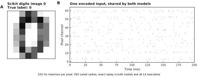
A: original image and label, displayed with inverted grayscale. B: its saved 200 ms encoding across 64 pixel channels. The annotation reports the input audit and maximum pixel rate. Arrivals retain the fixed 0.2 ms encoding grid.
COBA
COBA’s median E-neuron voltage difference outside spike windows fell from 1.62 to 0.2 mV between 0.1 and 0.0125 ms (Figure 2E). The continuous network emitted 3923 hidden E spikes. COBA has no inhibitory population.
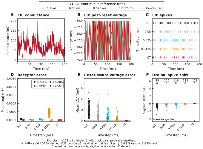
A–C: preselected E neuron 0. Continuous is red; AMPA is solid and GABA dashed. D–E: per-neuron receptor and voltage MAE outside inclusive ±2 ms windows around either train’s spikes. Circles are E; hollow D markers are GABA. F: signed median ordinal shifts for equal nonzero counts; labels give E above I eligibility counts. Black bars are population medians. Retained sample fractions appear below the panels. MAE means mean absolute error.
PING
PING’s median E-neuron voltage difference changed from 4.05 to 4.35 mV (Figure 3E); refinement of the discrete timestep did not reduce this error. At the finest timestep, the median I-neuron difference was 1.67 mV. The continuous network emitted 879 E/I spikes.
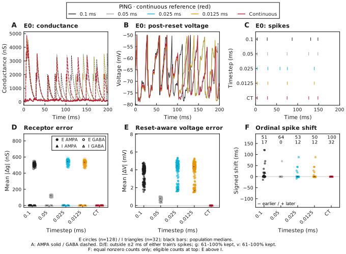
Same measurements as Figure 2, with active E→I→E feedback and a physical 0.2 ms recurrent delay. Triangles are I neurons. F excludes count mismatches and silence; equal counts alone do not establish spike identity. Output neurons do not enter these E/I error distributions.
Classification with matching output dynamics
Each discrete COBA-LIF output layer used its own network’s timestep: 0.1, 0.05, 0.025 or 0.0125 ms. In the continuous case, the output neurons evolved continuously alongside E/I. The saved native graph snapshots verify each discrete output clock; the continuous solver retains output threshold roots.
Both models selected the true digit in every condition (Figure 4). Continuous COBA predicted 0; continuous PING predicted 0. Class counts and ranks changed even though the winning digit did not. Total output spikes remain exp141’s trained class score.
Two separate 25 Hz source controls reproduced every saved exp141 spike and class score exactly. They are retained as validation evidence; all conditions in Figure 4, including the native 0.2 ms cases, use 100 Hz. Continuous refinement preserved every neuron’s count and all ten class counts; the largest root shift was 2.59e-11 ms. This is one training image, not a test-accuracy estimate or evidence of equivalent trajectories.
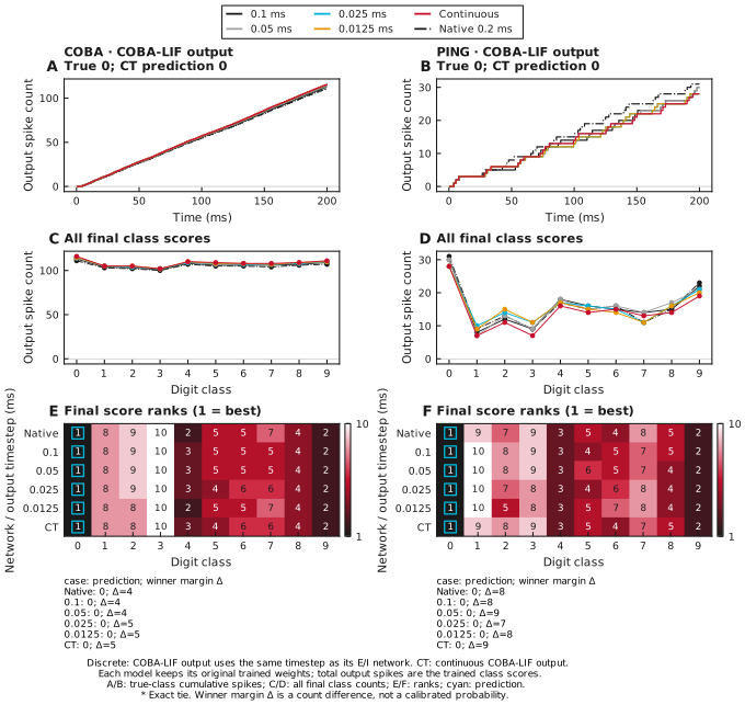
A–B: cumulative true-class output spikes, sampled at 0.1 ms for the sweep and continuous case; the native case retains its 0.2 ms clock. All use the same 100 Hz input encoding. C–D: all final class counts. E–F: class ranks, with cyan boxes marking the prediction. Rows include native 0.2 ms inference, four discrete cases and CT (continuous time). The listed winner margin is a spike-count difference. Exact ties select the lowest class index and receive an asterisk. Counts and margins are not calibrated probabilities.
Methods
- Select and verify the source (Figure 1). Pin
exp141-r012-computeby its payload digest. Load its native best-validation simulation-start parameter snapshots, rather than final-epoch weights. Replay the original saved 25 Hz input in separate controls and verify every hidden, inhibitory and output spike and score against the saved original. Encode the same image once at 100 Hz with the native SNNLab rate encoder. - Match physical arrivals (Figures 2–4). Use a 0.1, 0.05, 0.025 and 0.0125 ms sweep. Replay the same saved integer-nanosecond arrivals without rounding or resampling, including each graph’s spiking output layer at that same timestep. Preserve a physical 0.2 ms E–I delay and zero additional E-to-output delay. Retain native 0.2 ms inference separately because its slot timing differs.
- Integrate continuous dynamics (Figures 2–4). Integrate every continuous COBA-LIF voltage adaptively, with analytic receptor decay, full-weight arrivals, upward threshold roots, hard resets and exact refractory clamps. Retain all unrounded spikes and common 0.1 ms samples. Native-clock inference remains at 0.2 ms and uses the same 100 Hz input. See Appendix A for recording and arrival-clock conventions.
- Check numerical refinement (Figure 4). Tighten the tolerances and halve the maximum integration step. Require equal per-neuron and class counts, maximum root shift below 0.001 ms and maximum per-neuron guarded voltage MAE below 0.001 mV. Both models passed.
The input image, trained weights and spike-count scoring come from exp141. Inference uses a 100 Hz maximum pixel rate without retraining. Output dynamics follow the discrete or continuous condition being compared.
Continuous membrane equation
For membrane voltage in millivolts and time in milliseconds, all hidden, inhibitory and output neurons follow
is capacitance in nanofarads; , and are leak, AMPA and GABA conductances in microsiemens. Their reversal potentials , and are in millivolts. Receptors decay exponentially between arrivals. Each arrival adds its frozen weight to the appropriate conductance. Upward threshold crossings emit spikes, reset voltage and begin a physical refractory clamp; conductances keep evolving. Output neurons receive AMPA only and have the hidden E-cell physics. DOP853 integrates voltage between arrivals and threshold events. The parameter table records nominal and refined tolerances and step limits; recording times are independent of adaptive integration steps.
Appendix A — Recording and clock conventions
A1 — Output clock
Both architectures use a discrete COBA-LIF output layer on the same graph clock as their hidden neurons, or a continuous COBA-LIF output population. Native clock values below are verified against the executed SNNLab snapshots; CT means continuous time. Output spike counts remain the class score throughout.
| Condition | Network timestep (ms) | Output timestep (ms) |
|---|---|---|
| Native inference | 0.20 | 0.20 |
| 0.1 ms | 0.10 | 0.10 |
| 0.05 ms | 0.050 | 0.050 |
| 0.025 ms | 0.025 | 0.025 |
| 0.0125 ms | 0.013 | 0.013 |
| CT | continuous | continuous |
A2 — Input alignment and recording
The sweep uses 0.1, 0.05, 0.025 and 0.0125 ms timesteps. SNNLab generates one encoding at a 100 Hz maximum pixel rate on a fixed 0.2 ms grid, so every arrival lies exactly on every numerical clock. We compare the resolved input coordinates against the saved schedule and retain their checksum and zero timing error for every execution. Input spikes are neither regenerated nor rounded when changing the timestep. A separate replay of the saved 25 Hz encoding validates the original trained model and does not enter these plots.
Sweep and continuous states share a 0.1 ms recording clock. Native-clock inference retains its 0.2 ms clock and the same 100 Hz encoding. Its error statistics select the continuous reference’s exact existing 0.2 ms sample times, without interpolation. All spike timestamps retain their original resolution.
A3 — Arrival clocks
SNNLab labels conductance by the start of a slot and voltage/spikes by its end.
A recurrent projection with declared delay therefore has end-clock lag
, where is the numerical timestep. Matched E–I edges declare
. The matched hidden-to-output edge uses one slot, giving
zero additional physical lag. The native 100 Hz case preserves the trained
graph’s
same-slot readout and one-slot E–I edges; its E–I end-clock lag is zero and its
readout starts within the same integration slot as the hidden spike. These
native timings are retained separately from the physical-delay comparison.
The original 25 Hz reproduction controls remain separate validation evidence.
Refractory timing retains the source’s native
following_steps convention in discrete executions.
The continuous reference implements the physical-delay convention. Its numerical refinement establishes local solver stability for this input; it does not establish convergence of the discrete recurrent trajectories.
A4 — Retained voltage samples
For each neuron, the voltage-error calculation excludes inclusive ±2 ms windows around either train’s spikes. Entries below are the median retained sample fraction across each population. Error medians describe these retained samples; they are not full-waveform errors.
| Model | Timestep (ms) | E retained | I retained | Readout retained |
|---|---|---|---|---|
| COBA | 0.10 | 26.2% | absent | 1.6% |
| COBA | 0.050 | 30.8% | absent | 1.6% |
| COBA | 0.025 | 33.0% | absent | 1.6% |
| COBA | 0.013 | 34.9% | absent | 1.6% |
| PING | 0.10 | 96.0% | 61.3% | 62.1% |
| PING | 0.050 | 96.0% | 69.5% | 71.0% |
| PING | 0.025 | 96.0% | 63.1% | 62.1% |
| PING | 0.013 | 96.0% | 63.3% | 62.6% |
Network diagrams
The diagrams come from the actual matched 0.1 ms SNNLab bundles. Delay changes reuse each architecture’s diagram; the readout is a COBA-LIF population in both. Here denotes pixel input, the hidden populations and the readout. Every projection is labelled , with target first and source second. Arrowheads show excitation; bars show inhibition. Recording aliases and spike-count reductions are omitted.
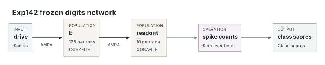
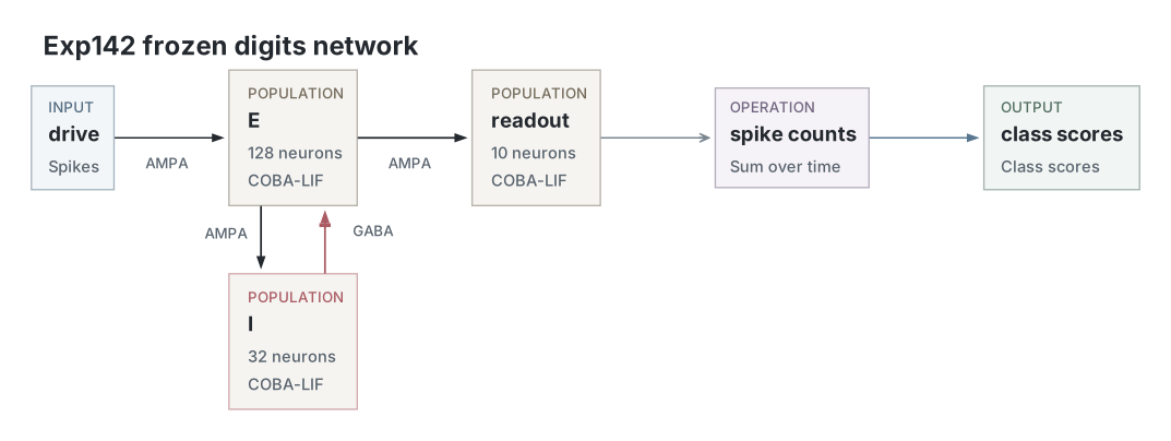
A: COBA. B: PING. The native circuit views retain each model’s own trained input and output weights. The output population shares its graph’s timestep. Matched recurrent declarations add one timestep to the physical 0.2 ms delay; the E-to-output declaration gives zero additional physical lag.
Parameters
Parameters are read directly from the native simulation-start snapshots in the selected compute run. E / I means excitatory / inhibitory; — denotes an absent population. Output cells use the E-cell membrane settings. Passive time constants are derived as capacitance divided by leak conductance. AMPA and GABA denote excitatory and inhibitory receptors. Matrix shapes come from the saved parameter inventory. Native delays refer to the 0.2 ms case; matched declarations are specified in A3.
| Parameter | COBA | PING |
|---|---|---|
| Network | ||
| Input channels | 64 | 64 |
| Population size, E / I | 128 / — | 128 / 32 |
| Output neurons | 10 | 10 |
| Neurons | ||
| Membrane model, E / I | coba_lif / — | coba_lif / coba_lif |
| Initial voltage, E / I | -65 / — mV | -65 / -65 mV |
| Passive time constant, E / I (derived) | 20 / — ms | 20 / 5 ms |
| Capacitance, E / I | 1 / — nF | 1 / 0.5 nF |
| Leak conductance, E / I | 0.05 / — µS | 0.05 / 0.1 µS |
| Resting potential, E / I | -65 / — mV | -65 / -65 mV |
| Reset potential, E / I | -65 / — mV | -65 / -65 mV |
| Spike threshold, E / I | -50 / — mV | -50 / -50 mV |
| Refractory period, E / I | 1.2 / — ms | 1.2 / 0.6 ms |
| Synapses and weights | ||
| Input→E receptor / decay (ms) | ampa / 2 | ampa / 2 |
| Input→E native declared delay (ms) | 0.0 | 0.0 |
| Input→E weight matrix shape | 64 × 128 | 64 × 128 |
| Input→E weights | Frozen validation-selected parameters | Frozen validation-selected parameters |
| E→output receptor / decay (ms) | ampa / 2 | ampa / 2 |
| E→output native declared delay (ms) | 0.0 | 0.0 |
| E→output weight matrix shape | 128 × 10 | 128 × 10 |
| E→output weights | Frozen validation-selected parameters | Frozen validation-selected parameters |
| E→I receptor / decay (ms) | Not applicable | ampa / 2 |
| E→I native declared delay (ms) | Not applicable | 0.20 |
| E→I weight matrix shape | Not applicable | 128 × 32 |
| E→I weights | Not applicable | Frozen validation-selected parameters |
| I→E receptor / decay (ms) | Not applicable | gaba / 6 |
| I→E native declared delay (ms) | Not applicable | 0.20 |
| I→E weight matrix shape | Not applicable | 32 × 128 |
| I→E weights | Not applicable | Frozen validation-selected parameters |
| Input and simulation | ||
| Maximum pixel input rate (Hz) | 100 | 100 |
| Training input rate (Hz) | 25 | 25 |
| Encoding seed | 0.0 | 0.0 |
| Input grid (ms) | 0.20 | 0.20 |
| Recording interval (ms) | 0.10 | 0.10 |
| Presentation (ms) | 200 | 200 |
| Discrete timesteps (ms) | 0.1 / 0.05 / 0.025 / 0.0125 | 0.1 / 0.05 / 0.025 / 0.0125 |
| DOP853 relative / absolute tolerance | 1e-8 / 1e-9 | 1e-8 / 1e-9 |
| DOP853 maximum step (ms) | 0.050 | 0.050 |
| Refined relative / absolute tolerance | 1e-10 / 1e-11 | 1e-10 / 1e-11 |
| Refined maximum step (ms) | 0.025 | 0.025 |
| Readout | ||
| Class score | Total output spikes; lowest index wins ties | Total output spikes; lowest index wins ties |
| Frozen checkpoint | validation_selected | validation_selected |
| Training | ||
| Training in this experiment | None; frozen inference | None; frozen inference |
| Source compute | exp141-r012-compute | exp141-r012-compute |
| Analysis | ||
| Spike exclusion window (ms) | ±2, inclusive | ±2, inclusive |
| Reference | Continuous, nominal tolerances | Continuous, nominal tolerances |
| Ordinal timing eligibility | Equal nonzero per-neuron counts | Equal nonzero per-neuron counts |
| Refinement maximum root shift (ms) | 0.0010 | 0.0010 |
| Refinement maximum guarded voltage MAE (mV) | 0.0010 | 0.0010 |
Dataset
Upstream: exp141 — Scikit-learn Digits
Downstream: —
Current runset
| Run | Date | Duration | Size | Evidence | Storage | Ran on | Verification |
|---|---|---|---|---|---|---|---|
| exp142-r026-present | 3s | 2.3 MB | Current | Both | Local | Local: byte-verified; R2: catalog-verified | |
| exp142-r025-analyse | 3s | 65.1 MB | Current | Both | Local | Local: byte-verified; R2: catalog-verified | |
| exp142-r024-compute | 23s | 48.3 MB | Current | Both | Local | Local: byte-verified; R2: catalog-verified | |
| exp141-r012-compute | 21m 9s | 907.4 KB | Current | Both | Local | Local: byte-verified; R2: catalog-verified |