AI to PING transition
Reducing external excitation of inhibitory neurons produces population oscillations in a conductance network derived from exp145 with fixed sparse input connectivity.
Abstract
The full recurrent shared-input conductance network runs through three windows: an AI target, an AI-to-PING transition, and a PING target. Only direct external excitation of inhibitory neurons is reduced; source rate, Input→E gain and all recurrent weights remain fixed from initialization. An unfitted four-state mean-field extension also predicts an oscillatory loss of equilibrium stability as Input→I strength decreases. This single-seed comparison does not establish an AI state or a PING mechanism.
Results
Median E-volley spacing in the final hold is 12.0 ms in its first 100 ms and 18.5 ms in its last 50 ms, using locally detected peaks. The full-window spectrum combines this evolution.
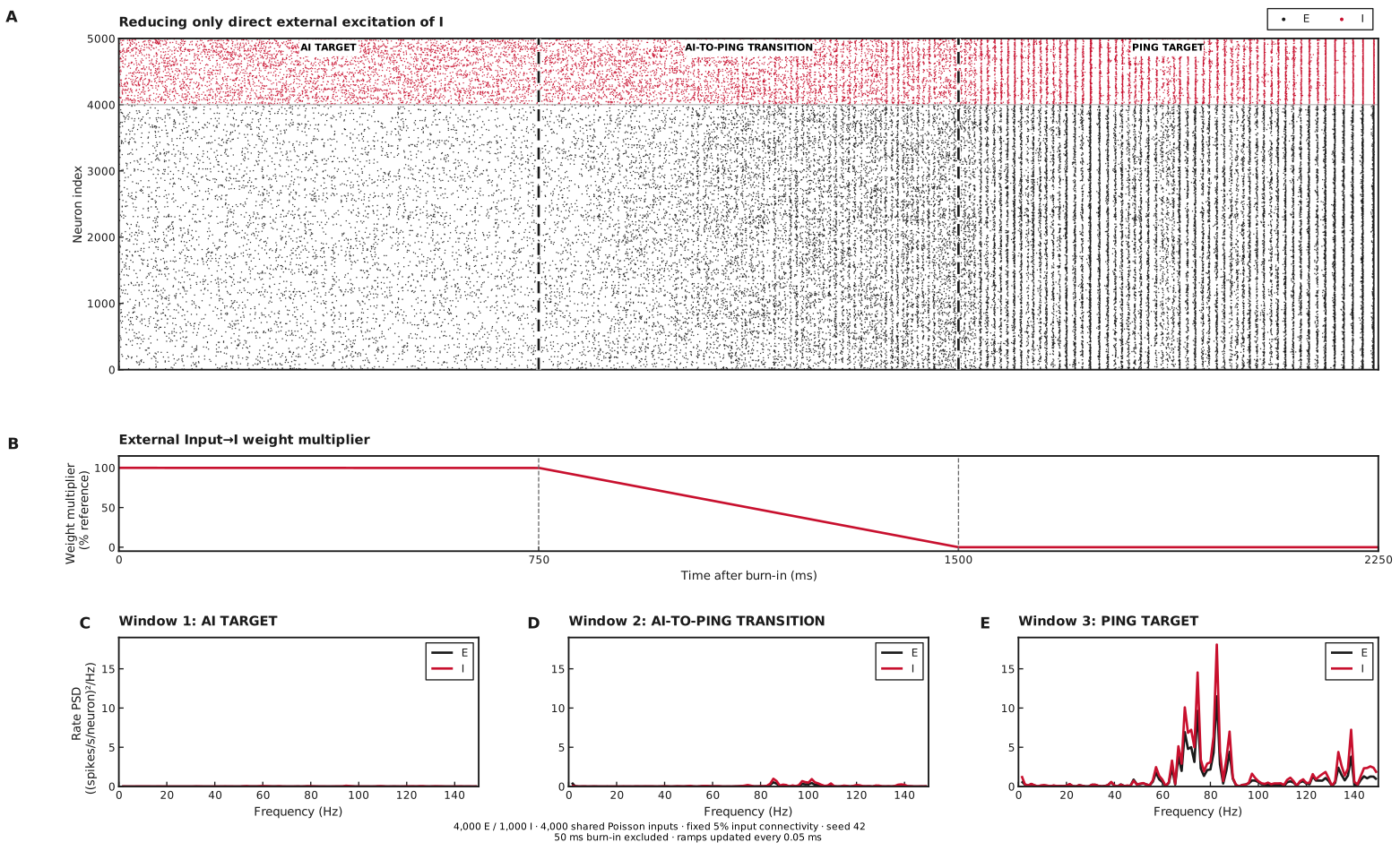
A: E spikes (black) and I spikes (red); three 750 ms windows after 50 ms burn-in. In all three windows, source rate stays at 2.5 Hz/source, Input→E gain and all recurrent gains stay at 100%. B shows the external Input→I weight multiplier falling from 100% to zero during window 2. C–E: population-rate spectra for windows 1, 2 and 3 (0.5 ms bins, Hann periodograms, 1.33 Hz spacing). All axes are linear. This runset contains the reference trajectory without input–output sweeps or pathway ablations.
Four-variable mean-field prediction
The displayed mean-field evidence precedes the SNNLab 0.27 migration. The current native implementation has not regenerated this trajectory; long onset trajectories can differ in phase with numerical tolerances.
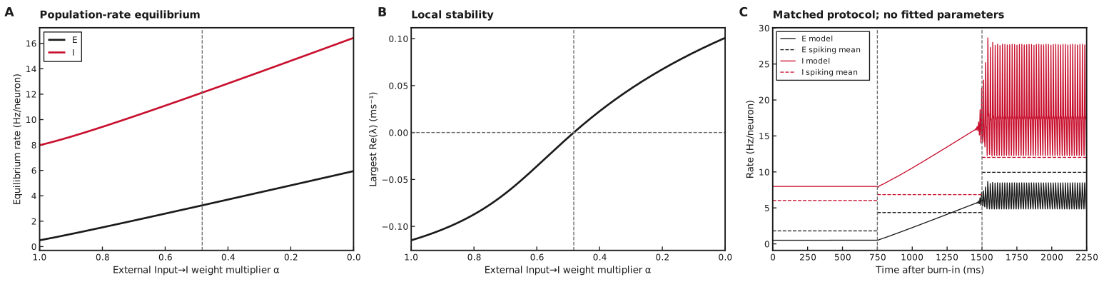
A: equilibrium E/I rates continued along decreasing Input→I weight multiplier. B: largest real part of the four flow-Jacobian eigenvalues; negative values indicate local stability. Vertical dashed lines in A/B mark the refined crossing. C: deterministic model rates (solid), with the observed spiking mean rates in each window (dashed). The model starts at its equilibrium with a small E-rate perturbation; its initial state differs from the spiking circuit’s resting-voltage initialization. The same 750 ms windows and linear weight schedule are used. The onset frequency is a linear stability estimate, not a fitted frequency of the finite-amplitude oscillation.
Model specialisation
We use the general mean-field model with all four recurrent pathways, shared input at spikes/source/ms (2.5 Hz/source) and no private input. All synaptic decays are 5 ms. Equilibrium-compatible initial conductances permit the note’s matched-decay four-state reduction, retaining despite nonzero self-coupling.
Only the Input→I matrix is multiplied by the scheduled gain ; Input→E and recurrence remain fixed. The model replaces changing external input by its instantaneous stationary mean, so the ramp’s filtering lag is omitted. Appendix D records the experiment-specific parameters, units, coupling provenance and numerical checks. The common conductance, current and gain derivations are in the note.
Calculations for Figure 2
-
Panel A — equilibrium rates. At 201 equally spaced multipliers from to zero, set all four time derivatives to zero and eliminate the recurrent conductances using the stationary filter relation. A star denotes equilibrium. Bounded least squares solves the stationary equations, using the preceding equilibrium as the next initial guess.
The earlier implementation eliminated conductances and required a maximum two-rate residual below 1e-7 Hz.Plot the resulting E/I rates against ; this continues one numerically found branch without establishing its global uniqueness.
-
Panel B — local stability. Write the four equations as , where and is the vector of time derivatives. Evaluate the analytical flow Jacobian at each equilibrium and plot , where are its four eigenvalues in ms. Negative values indicate local stability. Brent refinement locates the zero at 0.482. A complex pair crosses there while the other pair remains stable. Its linear onset frequency is 79.4 Hz, converting the critical eigenvalue’s imaginary part from radians/ms. This tests oscillatory onset without determining Hopf criticality.
-
Panel C — protocol integration. Start from the equilibrium, add spikes/neuron/ms to , and integrate the four equations through 50 ms burn-in and three 750 ms windows. Hold , decrease it linearly to zero in the middle window, then hold zero. Sample model rates every 0.5 ms; solver settings are in Appendix D. For each dashed spiking mean, count spikes within that window and divide by population size and its 0.75 s duration. These means are comparisons, not fitting targets.
Numerical settings and validation checks are recorded once in Appendix D. The closure’s oscillatory onset does not establish microscopic AI firing or the spiking network’s PING mechanism.
A. Network
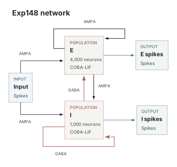
Native circuit diagram from the compiled graph used for this run. The native gain schedule scales only new Input→I drive. Input→E and all four recurrent pathways retain their reference weights from initialization. The same input pool, sampled weight matrices and connection masks are used throughout. denotes the shared external input pool. Every connection is labelled , with target first and source second. Arrowheads denote excitation; bars denote inhibition. Recording aliases are omitted.
B. Parameters
| Parameter | Value |
|---|---|
| Network | |
| E / I neurons | 4000 / 1000 |
| Shared Input sources | 4000 |
| E→E autapses allowed | false |
| E→I autapses allowed | false |
| I→E autapses allowed | false |
| I→I autapses allowed | false |
| Input→E autapses allowed | false |
| Input→I autapses allowed | false |
| Neurons | |
| Neuron model, E / I | coba_lif / coba_lif |
| Capacitance, E / I (nF) | 0.25 / 0.25 |
| Leak conductance, E / I (µS) | 0.0167 / 0.0167 |
| Derived time constants, E / I (ms) | 14.9701 / 14.9701 |
| Resting potential, E / I (mV) | -70 / -70 |
| Initial voltage, E / I (mV) | -70 / -70 |
| Reset potential, E / I (mV) | -60 / -60 |
| Spike threshold, E / I (mV) | -50 / -50 |
| Excitatory reversal, E / I (mV) | 0 / 0 |
| Inhibitory reversal, E / I (mV) | -80 / -80 |
| Refractory duration, E / I (ms) | 2 / 1 |
| Refractory scheduling | following_steps |
| Synapses and weights | |
| E→E synapse / decay / delay (ms) | ampa / 5 / 1 |
| E→E modulation | None |
| E→E initializer / scaling | lower_clamped_normal / direct |
| E→E compensated initializer mean / SD (µS) | 0.000096 / 0.000048 |
| E→E connected Gaussian parent mean / SD (µS) | 0.00048 / 0.00024 |
| E→E realised nonzero mean (µS) | 0.000493176 |
| E→E initial zero fraction / realised nonzero fraction | 0.8 / 0.195526 |
| E→E realised mean / SD including zeros (µS) | 0.0000964284 / 0.000219657 |
| E→I synapse / decay / delay (ms) | ampa / 5 / 1 |
| E→I modulation | None |
| E→I initializer / scaling | lower_clamped_normal / direct |
| E→I compensated initializer mean / SD (µS) | 0.000192 / 0.000096 |
| E→I connected Gaussian parent mean / SD (µS) | 0.00096 / 0.00048 |
| E→I realised nonzero mean (µS) | 0.000986577 |
| E→I initial zero fraction / realised nonzero fraction | 0.8 / 0.195359 |
| E→I realised mean / SD including zeros (µS) | 0.000192737 / 0.000439253 |
| I→E synapse / decay / delay (ms) | gaba / 5 / 0.5 |
| I→E modulation | None |
| I→E initializer / scaling | lower_clamped_normal / direct |
| I→E compensated initializer mean / SD (µS) | 0.0016 / 0.0008 |
| I→E connected Gaussian parent mean / SD (µS) | 0.008 / 0.004 |
| I→E realised nonzero mean (µS) | 0.00822137 |
| I→E initial zero fraction / realised nonzero fraction | 0.8 / 0.195467 |
| I→E realised mean / SD including zeros (µS) | 0.00160701 / 0.00366098 |
| I→I synapse / decay / delay (ms) | gaba / 5 / 0.5 |
| I→I modulation | None |
| I→I initializer / scaling | lower_clamped_normal / direct |
| I→I compensated initializer mean / SD (µS) | 0.0016 / 0.0008 |
| I→I connected Gaussian parent mean / SD (µS) | 0.008 / 0.004 |
| I→I realised nonzero mean (µS) | 0.00821862 |
| I→I initial zero fraction / realised nonzero fraction | 0.8 / 0.195567 |
| I→I realised mean / SD including zeros (µS) | 0.00160729 / 0.00366074 |
| Input→E synapse / decay / delay (ms) | ampa / 5 / 1 |
| Input→E modulation | None |
| Input→E initializer / scaling | lower_clamped_normal / direct |
| Input→E compensated initializer mean / SD (µS) | 0.000216 / 0.000108 |
| Input→E connected Gaussian parent mean / SD (µS) | 0.00432 / 0.00216 |
| Input→E realised nonzero mean (µS) | 0.0044414 |
| Input→E initial zero fraction / realised nonzero fraction | 0.95 / 0.04884 |
| Input→E realised mean / SD including zeros (µS) | 0.000216918 / 0.00105767 |
| Input→I synapse / decay / delay (ms) | ampa / 5 / 1 |
| Input→I modulation | ramp_gain |
| Input→I initializer / scaling | lower_clamped_normal / direct |
| Input→I compensated initializer mean / SD (µS) | 0.000216 / 0.000108 |
| Input→I connected Gaussian parent mean / SD (µS) | 0.00432 / 0.00216 |
| Input→I realised nonzero mean (µS) | 0.0044408 |
| Input→I initial zero fraction / realised nonzero fraction | 0.95 / 0.048806 |
| Input→I realised mean / SD including zeros (µS) | 0.000216738 / 0.00105663 |
| Input and simulation | |
| External input | One Poisson raster shared by Input→E and Input→I |
| Fixed Input / recurrent connection probability | 0.05 / 0.2 |
| Constant rate per Input source (Hz) | 2.5 |
| External seed offset | 10000 |
| Timestep / duration (ms) | 0.05 / 2300 |
| Execution seed | 42 |
| Execution device | cpu |
| Requested compilation mode | Off |
| CPU threads | 1 |
| Spikes recorded | All E and I neurons; raw recording includes burn-in |
| Excluded burn-in (ms) | 50 |
| Measurement window (ms) | 2250 |
| Input-generation block length (steps) | 1000 |
| Training | None; gains follow prescribed native modulation |
| Control protocol | |
| Scheduled parameter | Input→I weight |
| Baseline / final gain | 1 / 0 |
| Absolute ramp start / end (ms) | 800 / 1550 |
| Native gain sampling interval (ms) | 0.05 |
| Baseline / ramp / hold (ms) | 750 / 750 / 750 |
| Analysis | |
| Population-count bin width (ms) | 0.5 |
| Minimum peak separation (ms) | 10 |
| Prominence fraction of maximum bin count | 0.2 |
E/I pairs are listed in that order. Network values and sampled reference-weight statistics come from the native simulation-start snapshot. Protocol and analysis values come from the same compute run’s recorded configuration. Initialization statistics describe the sampled target weights before scheduled multipliers. Stored parameter arrays remain at these reference values; all recurrent pathways are fully active from initialization. Input jumps are scaled to preserve expected total input conductance at the selected fixed input sparsity. Gaussian parent moments differ from realised moments because of lower clamping and excluded autapses. A final zero Input→I gain stops new external drive to I; accumulated conductance continues to decay.
C. Hold-window analysis
Pulse timing is measured independently in consecutive 100 ms intervals using 0.5 ms population-count bins, a minimum peak separation of 6 ms and prominence of 12% of the largest count in each interval. This local threshold retains small early volleys that the full-hold threshold can miss. Intervals crossing 100 ms boundaries are omitted. The last interval is shorter when the hold duration is not a multiple of 100 ms. These descriptive measurements do not establish a PING mechanism. Native recordings also retain population mean voltage and mean conductance for each pathway. This runset contains no pathway-ablation controls.
D. Mean-field parameters and numerical checks
The mean-field note gives the model, gain, analytical gain slope and four-state reduction. The main-text specialisation defines exp148’s pathways and Input→I gain schedule. No exp117 numerical results are scientific inputs.
All six matrix sums use the referenced native parameter snapshot, including zeros and excluded autapses; initializer means are not substituted. The gain uses exp148’s recorded capacitance, leak, reset/threshold voltages and refractory periods. Its fixed noise scale is mV and rate-relaxation times are ms and ms. For both target populations, mV and mV. These closure choices and couplings are not fitted to the observed transition. Explicit transmission delays and weight heterogeneity are omitted; the note describes the shared-input covariance and shunting approximations.
The note’s equations use spikes/neuron/ms. Exp148’s implementation and rate figures use Hz: rates and gains are multiplied by 1,000, and rate inputs to conductance filters are divided by 1,000. Solver tolerances below are stated in the implementation’s Hz units. The scheduled matrix gain acts on new external input; substituting its instantaneous stationary mean omits the 5 ms input-filtering lag during the ramp.
The current recipe uses SNNLab’s native NoisyLIF gain with 48-point
Gauss–Legendre quadrature, symbolic Jacobian, bounded equilibrium continuation
and Brent stability-crossing refinement. Its matched-decay reduction retains
and ; reconstructed self-pathway conductances must satisfy the
native model’s constraints. The recorded graph is copied before translating
only its Input→I modulation into an explicit numerical control. The original
spiking evidence remains unchanged.
The selected figure retains the numerical implementation recorded in its run. Earlier figures used the experiment’s local gain and Jacobian; those duplicate implementations and comparison references have been removed. Protocol tests now cover native model construction, modulation handling and exported units. A complex crossing is an onset candidate; it does not determine criticality.
LSODA uses relative tolerance and native absolute rate tolerance Hz. Conductance absolute tolerances multiply that rate tolerance by or , respectively, in µS/Hz. The maximum integration step is 0.5 ms.
Dataset
Upstream: —
Downstream: —
Current runset
| Run | Date | Duration | Size | Evidence | Storage | Ran on | Verification |
|---|---|---|---|---|---|---|---|
| exp148-r102-present | 1s | 3.6 MB | Current | Both | Local | Local: byte-verified; R2: catalog-verified | |
| exp148-r101-analyse | <1s | 195.1 KB | Current | Both | Local | Local: byte-verified; R2: catalog-verified | |
| exp148-r100-compute | 1s | 216.1 KB | Current | Both | Local | Local: byte-verified; R2: catalog-verified | |
| exp148-r091-compute | 2m 53s | 31.2 MB | Current | Both | Local | Local: byte-verified; R2: catalog-verified |